Guido's SSB Modulation - Analysis and Application

This blog post is "work in progress" and may be updated from time to time. 

The uSDX, is a microprocessor-based Software Defined Transceiver developed by Guido PE1NNZ that has a very interesting technique to generate the SSB transmission. The SSB signal is created by rapidly updating both the output frequency and the output power of a class-E driven Power Amplifier. This design results in a power-efficient and very simple low cost circuit:

That's it - that's the enter transmit circuitry to generate a 5W SSB signal! That's crazy, and so much simpler than the typicaly SSB modulation techniques.

Guido's approach is such an attractive idea that the QMX is adopting a similar SSB modulation method.

This blog post describes my journey learning about this modulation technique, how it works, what its limitations are, and how those limitations can be minimised in a practical implementation. The journey I took led me down many blind alleys. I'll try to spare you from these, and try to chart a more direct and logical path.

My first step was to explore how it was even possible for this approach to modulate typical audio inputs. Understsanding it for a single input tone is easy - the output frequency and output power are just kept constant. For instance, if the transceiver is tuned to 7MHz upper sideband, and a modulating tone of 1kHz is applyed, the radio sets the si5351 CLK2 output frequency to 7.001MHz, and the PA amplitude to a value proportional to the input signal's amplitude. If the frequency or amplitude of the single tone modulating input changes, the output frequency and amplitude are updated accordingly.

When two audio signals, say at 1kHz and 1.9kHz, are applied then the output to the antenna should comprise two frequencies - one at 7.001MHz and one at 7.0019MHz. How is this possible when the transmitter is only capable of generating one frequency at a time? Well, it turns out that it is possible - by varying both the output frequency and output amplitude in exactly the right way. This can be shown mathematically in my blog post here.

I've gone on to confirm in both simulation software and laboratory-style tests that indeed a two frequency output signal can be accurately generated using Guido's modulation technique. However there are limitations to this approach which I will summarise here, and will explain later how I arrived at these conclusions.

Summary of Findings

The Guido modulation algorithm is nonlinear, and becomes increasingly nonlinear as the amplitudes of two input tones approach each other.  When this happens, as with any nonlinear system, many harmonics are generated and these harmonics are at frequencies that are multiples of the difference-frequency of the input tones. For example, if the input signals are at 1kHz and 1.9kHz, the difference frequency is 900Hz, and there are harmonics at 1800Hz, 2700Hz, 3600Hz, etc.

The harmonics are critical to the correct generation of the RF output. By "magic" the harmonics generated by the frequency variations exactly cancel the harmonics generated by the amplitude variations, resulting in a clean RF signal. Any reduction of the harmonic signals that are caused by bandwidth limitations in either the frequency or amplitude paths will result in spurious signals in the output.

A rough rule of thumb for the case of equal-amplitude input signals is that the bandwidth of the frequency and amplitude paths need to be approximately 5x the maximum expected frequency-difference in order to keep the output's spurious signals more than 30dB below either test tone. For instance, the si5351 can only be updated at about 12ksps maximum (with overclocking the I2C bus beyond spec), and so has a maximum bandwidth of 6kHz. Such a system will show spurious signals of worse than 30dB whenever equal-amplitude dual-tone signals are applied that have a freequency difference greater than \(\frac{6kHz}{5} = 1200Hz\).

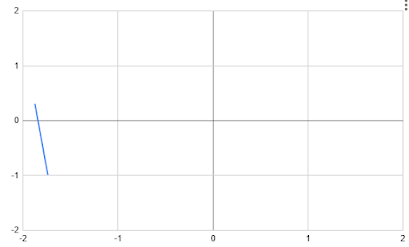
To illustrate the consequences of limiting the bandwith, here is the simulation result of a 6kHz bandwidth limitation on 300Hz and 1600Hz tones (1300Hz frequency difference) is:

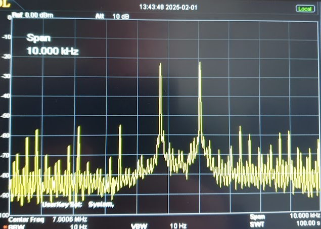
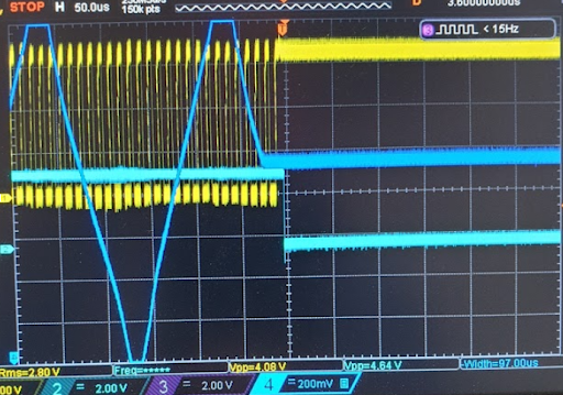
The same test on a laboratory hardware test set-up is:

Note the very strong similarity between the simulated results and real results (allowing for slightly difference horizontal and vertical scales). This is positive evidence of the accuracy of the simulation and my understanding of what is happening.

The Modulation Algorithm

The modulation algorithm at a high level is:

Or in pseudo-code:

modulate(audio): 

     (I, Q) = HilbertTransform(audio)

amplitude = sqrt(I*I, Q*Q)

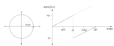
phase = atan2(Q, I)

deltaPhase = phase - lastPhase    // differentiate

lastPhase = phase

if (deltaPhase < 0)  deltaPhase = deltaPhase + 2*PI    // phase unwrapping

if (deltaPhase >PI) deltaPhase = deltaPhase - 2*PI     // phase unwrapping

frequency = deltaPhase * Const + CarrierFrequency

return (frequency, amplitude)

You might rightly wonder what is happening here - this is a huge jump from the description so far and from the mathematical analysis referred to above.

To understand how this algorithm works it helps to first describe:

1. The phasor representation of a sinusoid. 
2. The Hilbert transform, as it applies in this narrow application.
3. Phase unwrapping.

Phasor Representation

The key idea is that, since a sinusoid has both an amplitude and a phase, it can be represented as a vector(arrow) or phasor in a 2D space. The phasor's length is it's amplitude, and it's frequency is how quickly it rotates around it's "tail" in this 2D space. So the tip of a phasor representing a single tone traces a circle in this 2D space. The horizontal component of this phasor is the level of the signal we see. This is illustrated here.

At any point in time the phasor has a length (the distance from its tail to its tip) and an angle, which is the phasor's angle to the horizontal.

If a signal comprises multiple sinusoids, all the phasors representing these sinusoids are added together tip-to-tail, with each phasor continuing to rotate around its own tail. The result is a new result phasor with its tail at the origin and a tip that traces out a complex pattern in 2D space.

The resulting path could also be traced out by a hypothetical signal generator whose output amplitude and frequency is continually and precisely varied to match. The signal generator's output amplitude is the length of result phasor, and its frequency is the rate of change of the result phasor's angle. This is exactly the calculation being performed in the modulation algorithm!

The Hilbert Transform

The discussion above describes the use of phasors, but the input signal isn't in phasor form. That's where the Hilbert Transform (or Hilbert Filter) comes in - it turns the input into phasor form!

The Hilbert Transform takes an input sinusoid and through "magic" (which I don't understand) outputs two sinusoids I and Q, with Q delayed by exactly 90° compared to I. I and Q are the two dimensions of the 2D phasor space!

The Hilbert Transform is also linear, so if two sinusoids are combined and fed into the Hilbert Transform, the result is exactly the same as feeding each sinusoid into a separate Hilbert Transform and adding the result. ie 𝓗(a + b) = 𝓗(a) + 𝓗(b). This means we can feed our input signal, which comprises multiple frequencies, into the Hilbert Transform and the resulting I and Q signals correctly represent the result phasor described earlier.

Phase Unwrapping

We're almost there! The last issue to deal with is that the phase measurement only gives a raw value between -π and +π. But the actual phase angle of a sinusoid continues to grow without bound. This becomes an issue when we calculate the frequency by measuring the phase's rate of change.

If the raw atan2() phase value is used, the frequency calculation is incorrect each time the phase increases beyond π and jumps back to -π. That's why the following code is needed to "unwrap" the phase and to give the correct phase difference:

if (deltaPhase < 0)  deltaPhase = deltaPhase + 2*PI    // phase unwrapping

It is also possible for the phase be decreasing and for the phase to jump from -π to +π. The code to "unwrap" this case is:

if (deltaPhase >PI) deltaPhase = deltaPhase - 2*PI     // phase unwrapping

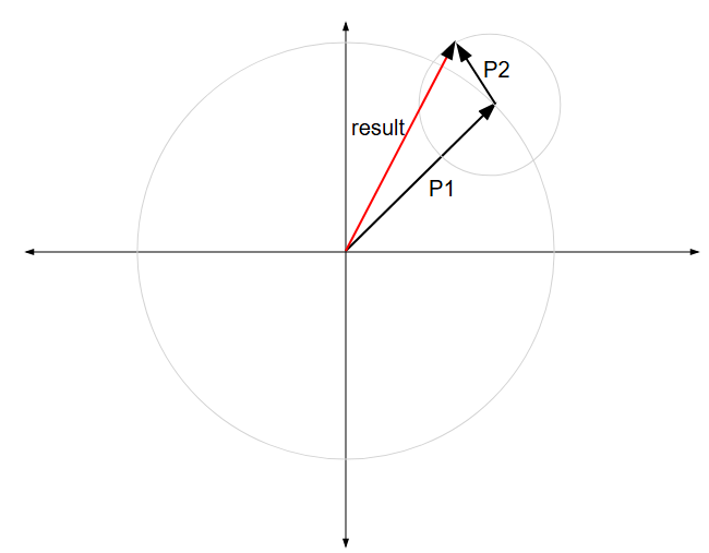
"When can the phase be decreasing - that's a negative frequency!" you might ask. Here's an example. Phasor 1 is rotating slowly (say at 100Hz), and Phasor 2 is rotating quickly (say at 1kHz). In the time that Phasor 2 rotates from position 1 to position 2 Phase 1 has hardly moved. The result phasor has reduced in phase:

This latter case of phase unwrapping is absent from the uSDX implementation, but appears to make little difference to the final signal because there is a relatively low proportion of time where negative phase happens simultaneously with encountering the phase discontinuity.

 Conclusion

This post has hopefully given some intuition behind Guido's modulation technique. In a subsequent post I'll investigate the the bandwidth requirements via simulation and a hardware implementation.

Mathematical Analysis of a two-tone SSB Signal

Suppose we have an SSB Transmitter tuned to transmit at carrier frequency \(f_c\), upper sideband. With an input audio modulating signal of \(f_a\), the transmitter generates an output signal of \( f_c + f_a\). For example if the tuned frequency is 7.0MHz and the audio input is 1kHz, a signal at 7.001MHz is generated.

Similarly, two input audio modulating signals \(f_a\) with amplitude a, and \(f_b\) with amplitude b, the transmitter generates a signal comprising two frequencies, one at \( f_c + f_a\)  and another at \( f_c + f_b\).

The following analysis shows that this 2-frequency output signal can be generated by amplitude-modulating an a single frequency-modulated oscillator. 

The following trigonometric identities are used:

(I): \( \cos(x+y) = \cos x\cos y - \sin x\sin y\) -- link

(II) \(x\cos\theta + y\sin\theta = c\cos(\theta+\phi)\) where \( c = sgn(x)\sqrt{(x^2+y^2)}\), \(\phi = \arctan(-y/x)\) -- link

(III) \( \sin^2x + \cos^2x = 1\) -- link

We start with the output signal:

\( s = a\cos 2\pi(f_c+f_a)t + b\cos 2\pi(f_c+f_b)\)

Define \( \omega_c = 2\pi f_c \),  \(\omega_a = 2\pi(f_c+f_a)\) and \(\omega_b = 2\pi(f_c+f_b)\):

\( s  = a\cos \omega_a t + b\cos \omega_b \)

\( s = a\cos \omega_a t + b\cos (\omega_a t + (\omega_b - \omega_a) t)\)

Applying (I): 

\( s = a\cos \omega_a t + b \cos \omega_a t \cos (\omega_b - \omega_a) t - b\sin\omega_a t \sin (\omega_b - \omega_a) t\)

Rearranging:

\( s = (a + b\cos (\omega_b - \omega_a) t) \cos\omega_a t  - b\sin\omega_a t \sin (\omega_b - \omega_a) t\)

Applying (II), with \(x = (a + b\cos (\omega_b - \omega_a) t)\), \(y = b\sin(\omega_b - \omega_a)t\):

\(s = \sqrt{a^2 + 2ab\cos(\omega_b - \omega_a) t + b^2\cos^2(\omega_b - \omega_a) t +  b^2\sin^2(\omega_b - \omega_a) t} \cos\left({\omega_a t  +\tan^{-1} \frac{b\sin(\omega_b - \omega_a) t}{a+b\cos(\omega_b - \omega_a) t}}\right)\)

Applying (III) to simplify the terms under the square root:

\(s = \sqrt{a^2 + 2ab\cos(\omega_b - \omega_a) t + b^2} \cos\left({\omega_a t  +\tan^{-1} \frac{b\sin(\omega_b - \omega_a) t}{a+b\cos(\omega_b - \omega_a) t}}\right)\)

This complex equation can be better understood by rewriting it as:

\(s = A \cos (\omega_a t  + f(t))\)

where:

• \( A = \sqrt{a^2 + 2ab\cos(\omega_b - \omega_a) t + b^2} \) sets the amplitude of the generated signal, and varies slowly compared to the carrier frequency because \( \omega_b - \omega_a \ll \omega_c\), and
• \( f(t) = \tan^{-1} \frac{b\sin(\omega_b - \omega_a) t}{a+b\cos(\omega_b - \omega_a) t} \) and varies slowly compared to the \(\omega_a t\) term, again because  \( \omega_b - \omega_a \ll \omega_c\).

In other words, combining two input signals results in an output signal with a phase varying around \(\omega_a t\) at the difference frequency \(\omega_b - \omega_a\) and with amplitude A also varying at the difference frequency.

Confidence that the formula is correctly derived can be gained by testing what happens if either of the modulating signals is removed (by setting it's amplitude term - either a or b - to zero. The formula should "collapse" to a single simple waveform. Indeed this is exactly what happens.

The analysis so far draws on "Frequency Analysis, Modulation and Noise", Standford Goldman, 1948 - p160. I believe what follows is novel.

Phase/Frequency Analysis

The full phase term is: \(\left({\omega_a t  +\tan^{-1} \frac{b\sin(\omega_b - \omega_a) t}{a+bcos(\omega_b - \omega_a) t}}\right)\).

The frequency at any instant in time is the derivative of this term with respect to time:

\( f = \frac{d}{dt}\left({\omega_a t  +\tan^{-1} \frac{b\sin(\omega_b - \omega_a) t}{a+b\cos(\omega_b - \omega_a) t}}\right)\)

\( f = \omega_a + \frac{d}{dt}\left({ \tan^{-1} \frac{b\sin(\omega_b - \omega_a) t}{a+b\cos(\omega_b - \omega_a) t}}\right)\)

Deriving the derivative of this second term is beyond my mathematics skills, but thankfully the Derivative Calculator website will do this for us (click the "Go!" button). Here I have defined \(m = \omega_b - \omega_a\).

The result is gives is: \(\frac{bm \left(a \cos\left(mt\right) + b\right)}{b \left(2a \cos\left(mt\right) + b\right) + a^{2}}\)

This formula isn't very informative, apart from showing that the output frequency varies with the difference frequency \(m = \omega_b - \omega_a\). However, very helpfully, Derivative Calculator also interactively plots the input and derivative values for the input values a, b and m. For example:

Experimenting with different values starts to give some slight intuition about how the amplitude values influence the frequency output. For instance, as the two amplitudes approach each other, the frquency variation grows dramatically:

Finally, when the two amplitudes are equal, there's a discontinuity & the "blip" disappears from the graph view - the negative "blip" is still there and corresponds to the negative edge of the input signal, but it's infinitely narrow and doesn't display:

This tendency for the frequency "blip" to grow without bound as one amplitude approaches the other is extremely important phenomena to understand in later analysis. It will also become apparent that this phenomena changes slightly when we move from the continuous domain to the discrete/sampled domain.

Note that the blue waveform might initially look strange when the amplitude is increased further:

The explanation for the discontinuities in the blue input waveform is that it is a phase measurement and has been displayed to wrap every \(2\pi\). The red derivative is displayed correctly and does not show any "blips" at these transitions.

Amplitude Analysis

The amplitude term is \( A = \sqrt{a^2 + 2ab\cos(\omega_b - \omega_a) t + b^2} \).

Its behaviour can be interactively plotted here.

The most interesting plot is again when \(a = b\):

This is a rectified sine wave, as can be demonstrated by setting \(a = b = 1\). The amplitude term simplifies to:

\( A = \sqrt{1 + 2\cos(\omega_b - \omega_a) t + 1} \)

\( A = \sqrt(2)\sqrt{1 + \cos(\omega_b - \omega_a) t } \)

But \(sgn(\cos\frac{\theta}{2})\sqrt{\frac{1 + \cos\theta}{2}}= \cos\frac{\theta}{2}\)  (see link).

So, ignoring the sign term, the amplitude is the shape of a cosine wave.

A rectified sine wave has high harmonic content (see here or here), which will become relevant in later analysis.

Conclusions

This mathematical analysis has derived some equations for both amplitude and frequency shift that appear to correspond to expectations.

The interactive waveform plots give some intuition on the signal behaviour. In particular, when the two tones approach the same amplitude, the frequency shift approaches a discontinuity and values can become very large, and the amplitude waveform approaches a shape that has high harmonic content.

 

Measuring the Si5351 Output Frequency Settling Time

 I'm using the Si5351 programable clock generator in an upcoming project, portions of which are similar to the usdx. For my application, characteristics of the chip that are important, but not documented in the datasheet, are:

• When does the output frequency change in relation to the I2C command that has been issued to update the frequency? Answer: on the second to last low-to-high I2C clock transition of the command that writes the lowest byte of the PLL register.
• How long does the output frequency take to reach the target frequency (its settling time)? Answer: < 1us! Yes, it settles extremely quickly.

This note describes how I measured these characteristics.

For my tests, the Si5351's output frequency is being updated at up to 12k times per second. The I2C bus is overclocked at 800kHz to achieve this update rate. The usdx project implements a frequency-change mechanism where just 5 on-chip 8-bit register values are updated in a single I2S 7 byte transaction. The update is made to alter the PLL frequency. For the purposes of my tests I use the same mechanism, but only need to update 4 registers for the range of frequency changes I'm conducting. Documenting the exact frequency update mechanism is outside the scope of this note, but can be ascertained from the usdx code and reference to AN619.

Note that my tests also showed that the Si5351 output only changes when the lowest byte of 

Test Method

I used a mixer to compare the Si5351's output target frequency against a known reference frequency. The filtered mixer's output is the difference between the input frequencies. So when the two frequencies are the same, or very similar, the output is either constant or changes only slowly. I initially used a filter RC time constant of 1us.

The mixer was built from a 3253 analogue switch. The mixer is very much like a quarter of a Tayloe Mixer.

The fixed frequency could be provided by an external source, but in my case I used a second Si5351 output.  I have relied on the fact that the si5351 can be configured to output 2 frequencies completely independently - each with their own PLL and MultiSynth divider chain (a third output frequency can also be configured, but must share one of the PLLs):

• the target frequency on CLK1 whose frequency will be adjusted by ±4kHz (or more).
• the reference frequency on CLK2 whose frequency is locked and stable throughout a test.

A Pi Pico 2 was used for generating the I2C signals, and output a "high" on a digital pin just before the start of a I2C transaction, and "low" immedately after. An oscilloscope monitored the I2C clock, the digital pin, and the mixer output.

To conduct the measurement, the target frequency would first be set several kHz above or below the reference frequency and allowed to stabilise, and then the target frequency would be set to match the reference frequency.

A typical trace (with the target frequency starting 5kHz above the target frequency, with C = 1nF & RC = 1us) is:

(where yellow = I2C clock, cyan = digital output, blue = mixer output).

The 5kHz difference frequency is clearly visible on the mixer output prior to the frequency change. The flat flat output after the frequency change shows that the target and reference frequencies are now equal.

Zooming in, we see that the mixer output becomes flat (ie target and reference frequencies now equal) within a few microseconds after the second to last low-to-high transition of the I2C clock. The 1us RC time constant of the filter slows the transition:

With C = 100pF, RC = 0.1us there is reduced filtering, but the exact time thta the frequency changed is much clearer:

The frequency transition occurs within 1us.

The tests were rerun using an external Function Generator as the reference frequency. The same results were obtained and verify that there was no unintentional interaction between the two Si5351 outputs.